Implementation of Bressenham's Line Drawing Algorithm

Implementation of Bressenham's Circle Drawing Algorithm

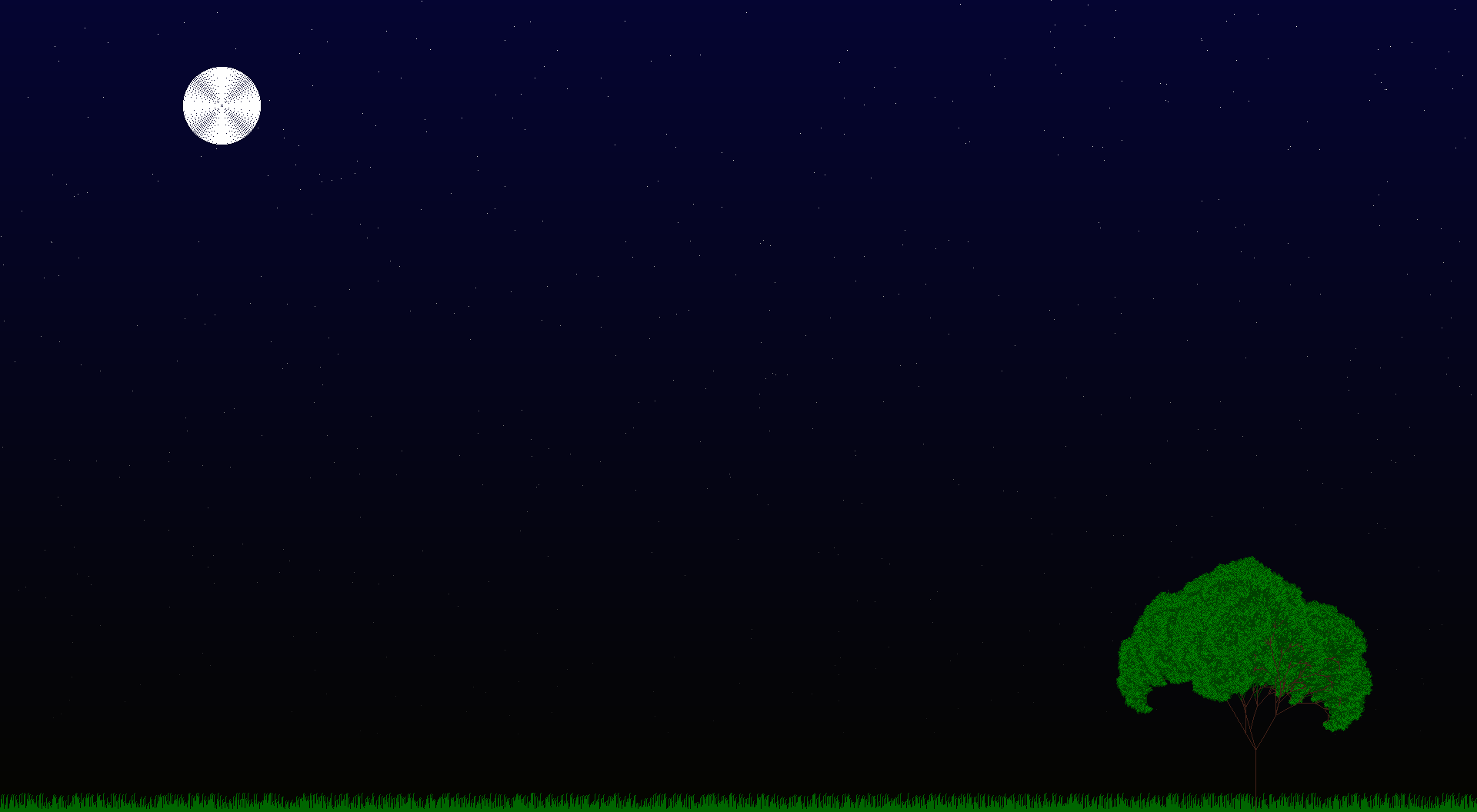
The recursive nature of the L-system rules leads to self-similarity and thereby, fractal-like forms are easy to describe with an L-system. Plant models and natural-looking organic forms are easy to define, as by increasing the recursion level the form slowly 'grows' and becomes more complex. Lindenmayer systems are also popular in the generation of artificial life.
The rules of the L-system grammar are applied iteratively starting from the initial state. As many rules as possible are applied simultaneously, per iteration. The fact that each iteration employs as many rules as possible differentiates an L-system from a formal language generated by a formal grammar, which applies only one rule per iteration. If the production rules were to be applied only one at a time, one would quite simply generate a language, rather than an L-system. Thus, L-systems are strict subsets of languages.
		variables : A B
		constants : none
		axiom  : A
		rules  : (A → AB), (B → A)
		which produces:

		n = 0 : A
		n = 1 : AB
		n = 2 : ABA
		n = 3 : ABAAB
		n = 4 : ABAABABA
		n = 5 : ABAABABAABAAB
		n = 6 : ABAABABAABAABABAABABA
		n = 7 : ABAABABAABAABABAABABAABAABABAABAAB
We followed two different approaches for constructing L-system based graphics.
Similar to the above example, each vaariable is recursively grown in each generation as per the given rule.
	variables : A
	constants : B
	axiom  : A
	rules  : (A → A[BA]A), (B → B)

	which produces:

	n = 0 : A
	n = 1 : A[BA]A
	n = 2 : A[BA][BA[BA]]A[BA]A
	n = 3 : A[BA][BA[BA]][BA[BA][BA[BA]]]A[BA]A[BA[BA]A]A[BA]A
Only the variables inside a subbranch are grown further. Variables in the main branch are not grown
	variables : A
	constants : B
	axiom  : A
	rules  : (A → A[BA]A), (B → B)

	which produces:

	n = 0 : A
	n = 1 : A[BA]A
	n = 2 : A[BA[BA]]A
	n = 3 : A[BA[BA][BA[BA]]]A
Implementation of Bressenham's Line Drawing Algorithm
Implementation of Bressenham's Circle Drawing Algorithm
Both the implementations yield different results because of the different growth pattern. So we tried different rules on different implementations and got some fascinating results. All such results are documented below.
	variables : F G
	constants : None
	axiom  : F
	rules  : (F → F+F-F-F-G+F+F+F-F), (G → GGG)

	which produces:

	n = 0 : F
	n = 1 : F+F-F-F-G+F+F+F-F
	n = 2 : F+F-F-F-G+F+F+F-F+F+F-F-F-G+F+F+F-F-F+F-F-F-G+F+F+F-F-F+F-F-F-G+F+F+F-F-GGG+F+F-F-F-G+F+F+F-F+F+F-F-F-G+F+F+F-F+F+...
	n = 3 : and so on
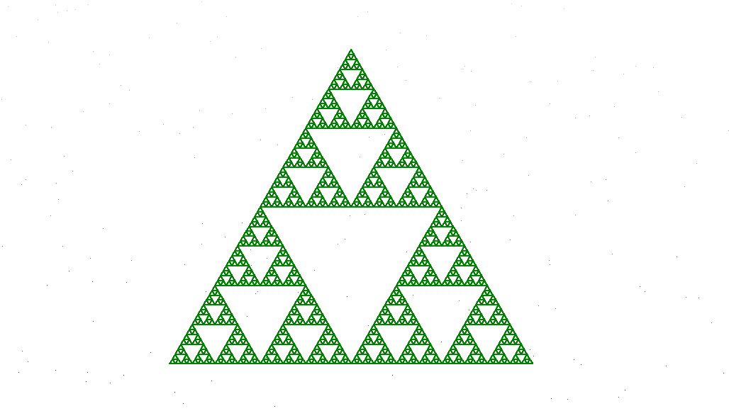
	variables : F
	constants : None
	axiom  : F-F-F-F-F
	rules  : (F → F-F++F+F-F-F)

	which produces:

	n = 0 : F-F-F-F-F
	n = 1 : F-F++F+F-F-F-F-F++F+F-F-F-F-F++F+F-F-F-F-F++F+F-F-F-F-F++F+F-F-F
	n = 2 : F-F++F+F-F-F-F-F++F+F-F-F++F-F++F+F-F-F+F-F++F+F-F-F-F-F++F+F-F-F-F-F++F+F-F-F-F-F++F+F-F-F-F-F++F+F-F-F++F-F++F+F-F-F....
	n = 3 : and so on
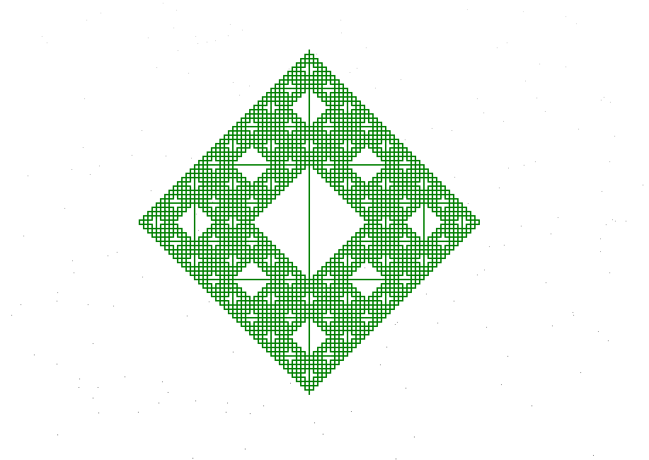
	variables : F G
	constants : None
	axiom  : F-G-G
	rules  : (F → F-G+F+G-F), (G → GG)

	which produces:

	n = 0 : F-G-G
	n = 1 : F-G+F+G-F-GG-GG
	n = 2 : F-G+F+G-F-GG+F-G+F+G-F+GG-F-G+F+G-F-GGGG-GGGG
	n = 3 : and so on
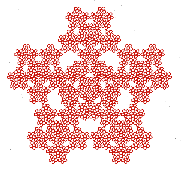
	variables : X F
	constants : None
	axiom  : X
	rules  : (X → [FFXFXFF][++XF][--XF]), (F → FC2cC0)

	which produces:

	n = 0 : A
	n = 1 [FFXFXFF][++XF][--XF]
	n = 2 [FC2cC0FC2cC0[FFXFXFF][++XF][--XF]FC2cC0[FFXFXFF][++XF][--XF]FC2cC0FC2cC0][++[FFXFXFF][++XF][--XF]FC2cC0][--[FFXFXFF][++XF][--XF]FC2cC0]
	and so on
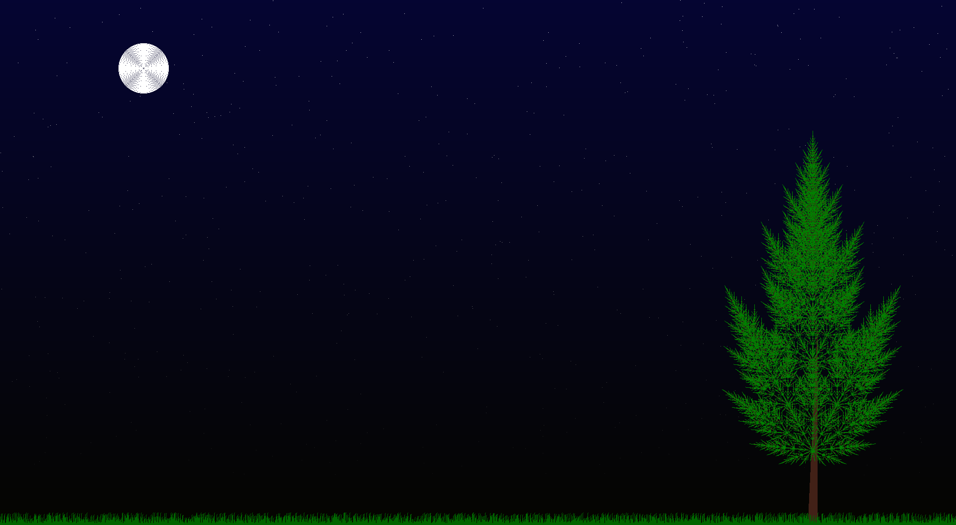
	variables : X F
	constants : None
	axiom  : X
	rules  : (X → F[FX][+FX][-C0cC2XF[X]]), (F → F[-XF])

	which produces:

	n = 0 : X
	n = 1 : F[FX][+FX][-C0cC2XF[X]]
	n = 2 : F[F[-XF]F[FX][+FX][-C0cC2XF[X]]][+F[-XF]F[FX][+FX][-C0cC2XF[X]]][-C0cC2F[FX][+FX][-C0cC2XF[X]]F[-XF][F[FX][+FX][-C0cC2XF[X]]]]
	and so on
	variables : X F
	constants : None
	axiom  : X
	rules  : (X → C2FC0[-X][+F[-X][FX]][F[-X][FX]]), (F → FFC1cC0)

	which produces:

	n = 0 : A
	n = 1 : C2FC0[-X][+F[-X][FX]][F[-X][FX]]
	and so on